With SQL server 2014 SP 2 Microsoft added a new feature that sounds pretty sweet for troubleshooting some performance problems. It is called Clone Database. In a Nutshell Clone database gives you a copy of the specified databases without any data in it, but with the statistics and heuristics of the database as if it did have data in it.

A script containing the code referenced in this post can be found here (dbcc-clone-db).

Some Quick Research

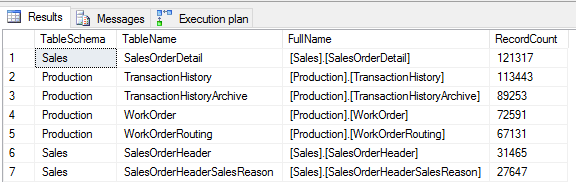
To start we will use AdventureWorks2014 database and find the largest table.

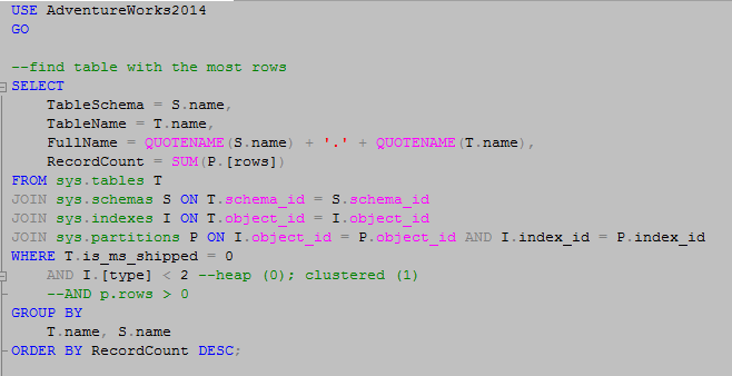
SalesOrderDetail has the most rows. It has enough rows to illustrate what I want to show in this article and we do not need to load more rows into it.

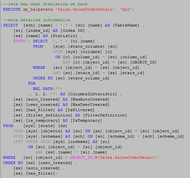
Let’s do a quick review the of indexes on the table to see what we have to work with

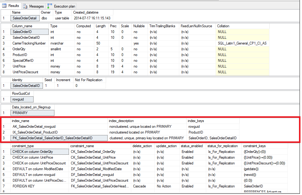
We can see we have indexes on rowguid, another on ProductId, and one using SalesOrderId and SalesOrderDetailId.

What statistics do we have on this table right now? There are a few ways to review this information.

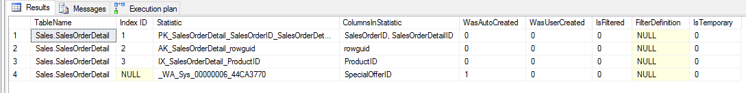
We can see there are statistics for each of our indexes and there are also some autocreated statistics on SpecialOfferId.

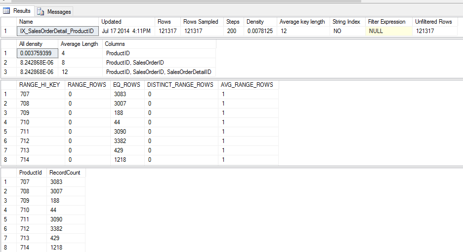
For our tests we will use ProductId. Let’s review its distribution.

As Erin Stellato stated in her blog on statistics (https://www.simple-talk.com/sql/performance/managing-sql-server-statistics/)

“The Updated column in the statistics header displays the last time statistic was updated, whether it was via an automatic or manual update. We can use the Rows and Rows_Sampled columns to determine whether the sample rate was 100% (FULLSCAN) or something less.

The density vector, which is the second set of information, provides detail regarding the uniqueness of the columns. The optimizer can use the density value for the left-based column in the key to estimate how many rows would return for any given value in the table. Density is calculated as “1/unique number of values in the column”.

The final section of the output, the histogram, provides detailed information, also used by the optimizer. A histogram can have a maximum of 200 steps, and the histogram displays the number of rows equal to each step, as well as number of rows between s

The teps, number of distinct values in the step, and the average number of rows per value in the step.”

 Looking at our density vector we have 0.003759399 or 265.999964 distinct values which we can check by running

SELECT DISTINCT ProductId FROM Sales.SalesOrderDetail –266 distinct ProductIds

Looking at our histogram we can see the RANGE_HI_KEY matches our ProductIds and EQ_ROWS matches the number of records corresponding to that ID

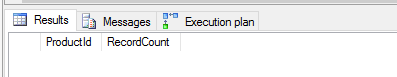
SELECT ProductId, COUNT(*) as RecordCount FROM Sales.SalesOrderDetail GROUP BY ProductId ORDER BY 1 ASC

The Setup

Now that we have researched some basic information. Let’s run some queries.

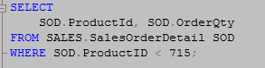
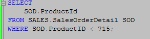
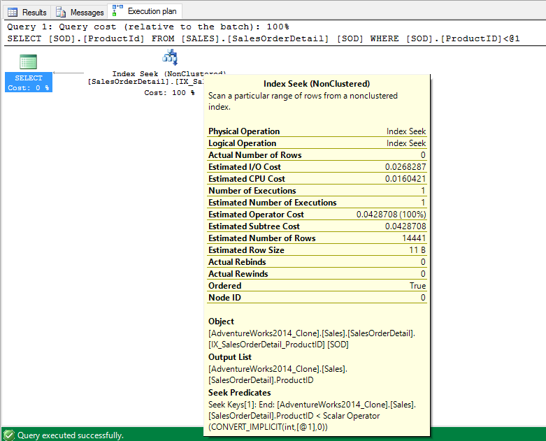
First we will run a query using ProductId in the where clause. Since ProductId is also the only column in our select list or joins from the SalesOrderDetail table we expect this will give us an execution plan using a seek operation.

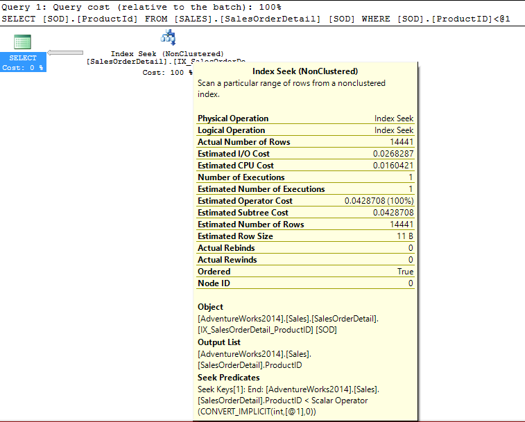
We can see the optimizer did indeed perform a seek using the IX_SalesOrderDetail_ProductId index.

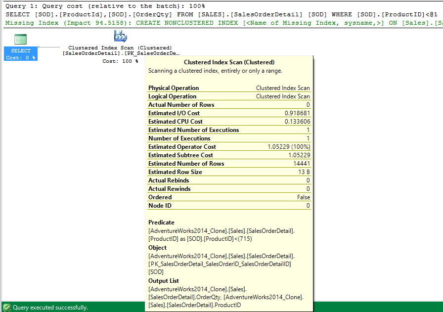
We will now add the OrderQty field to our requested output. Since this field is not in any indexes the optimizer will have to get it by either scanning an index or by doing a bookmark lookup against our clustered index. Since there are only 121317 records in the SalesOrderDetail table. We expect it will most likely choose to perform a clustered index scan. Let’s find out.

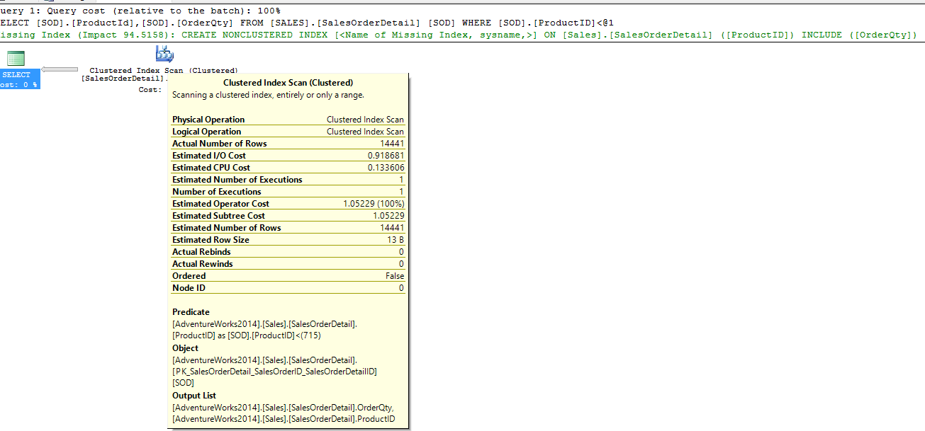
We did indeed get a clustered index scan.

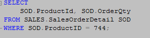
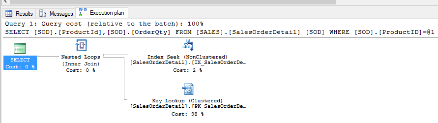
From our research above when we ran SELECT ProductId, COUNT(*) as RecordCount FROM Sales.SalesOrderDetail GROUP BY ProductId ORDER BY 1 ASC we found that ProductId 744 only had 13 records associated to it. With this small amount of records we should be able to see if we can get a seek and a lookup that is less costly than an index scan.

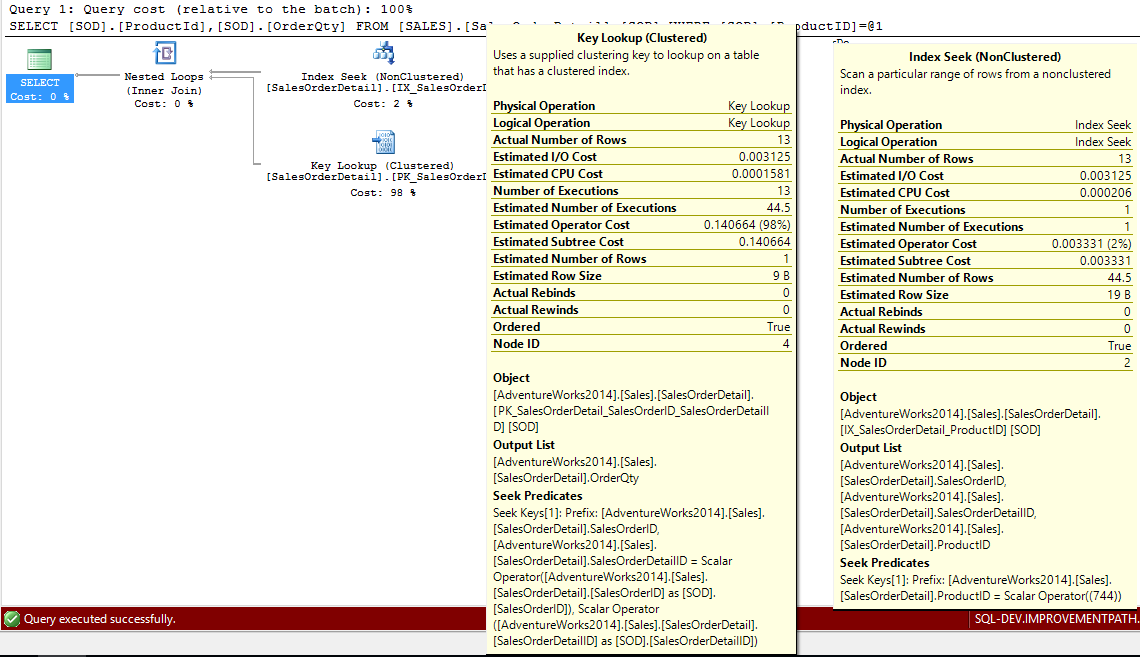
We did. Excellent.

In Comes Clone Database

That was a lot of setup. Now let’s bring in DBCC CloneDatabase and see what we can do what we can do with a database without any data in it.

Clone our AdventureWorks2014 database using the following command.

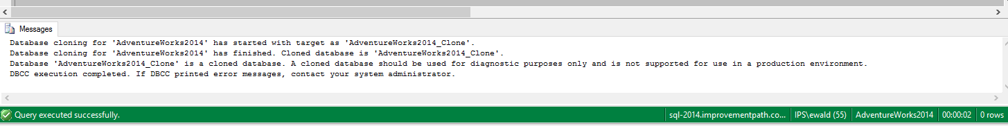
We can see it created our clone in readonly mode.

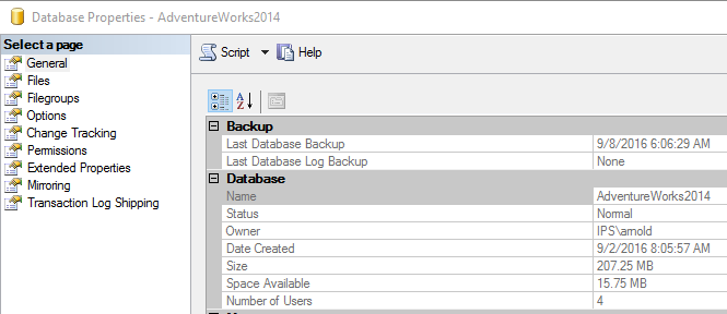
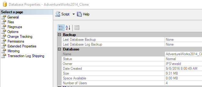
We can also see that it is significantly smaller.

Rerunning our query Some Quick Research # 1 over the clone copy we see we still get the same row counts for the tables since the query is based off of metadata.

Running a direct query from the table shows we do not actually have data however.

SELECT ProductId, COUNT(*) as RecordCount FROM Sales.SalesOrderDetail GROUP BY ProductId ORDER BY 1 ASC

Now let’s check our execution plans over the clone database. We expect the same plans.

The same Index Seek…

The same Clustered Index Scan…

The same index seek with bookmark lookup…

We can see that we got the same execution plans. Let’s try to create a covering index for query 2 to see if we can change it from a clustered index scan to an index seek. Remember there is no data in this database.

I want to create a covering index to test the results. Since we cannot create or alter an index on a database in read_only mode. Let’s see if it allows us to change that.

Now create a new covering index that includes both ProductId and OrderQty. Note: normally we would probably just add the OrderQty to the already existing ProductId index.

Now that the index is created lets run our query one last time to see if we get a different execution plan.

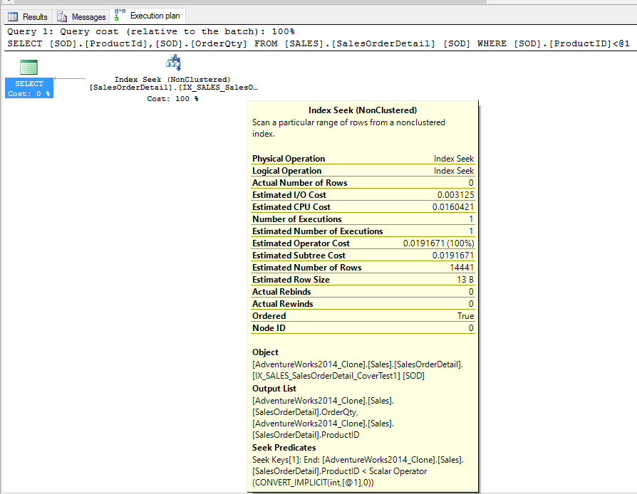
We can see the optimizer did use our new covering index to perform an index seek instead of just determining the clustered index scan was the most efficient way to go.

I can see clone database being a great tool in the toolbox.

Can you see fitting this into your troubleshooting routine?

Let us know in the comments below.